
Churn Modelling Part 3:
Model Implementation
“The secret to modelling…is to bring something new!” -Karl Lagerfeld
In Part 1 we discussed what churn modelling is in the wider context of time series data. In Part 2 we dove deep into the process behind constructing windows that allow us to run models effectively. In this third and final chapter of the beloved churn modelling trilogy, I will be talking about various aspects of model implementation.
Once the datasets are structured properly, the process of churn modelling isn’t too distinct from other methods of predictive classification, and indeed many ML best practises still apply. Nonetheless, churn modelling still offers some peculiar aspects that should be carefully considered to get the best out of your model. I will be touching on those points below.
Feature Types in Churn Modelling
There are various types of features that can be effectively included in your churn model. These can be designated as follows.
1. Static features
This is information that likely will not change much for the user over time. It might include such things as country of origin, gender, which plan they’re on, or whether they used a coupon to sign up or not.
Static information is useful as an easy way to broadly categorise users largely independent of when the model is run. This may provide important details in conjunction with the dynamic or period data that will make up the bread-and-butter of your model’s features.
One thing to be careful of is with static information is situations where most of the feature is made up of just one category. For instance, if 95% of your users are British, and most users do not churn in any given period, you don’t want to end up with the association that being British means users will not churn!
2. Dynamic features
This is information that is highly variable from user to user. It could include the frequency of activity on the website, responsiveness to prompts or emails, amount of money being spent on products, or number of times they’ve reached out to customer support. The data for this information could be aggregated or split up across the feature window (both methods covered in Part 2).
Dynamic information will be the core of your features since it’s the most effective way to distinguish two otherwise similar users. The key is to identify what features, and what arrangement of time periods, provides the strongest signals for your model. You might find for example, that heightened activity in a user’s final week on their plan is a strong indicator of churn, as users try to extract as much benefit as they can before leaving the product permanently. Or you might find the exact opposite!
3. Period features
This is information that is mutable (like dynamic information) but also predictable once established (like static information). It may include time since purchase of plan, number of renewals, or time till end of plan. Period information can offer useful information to your model; for instance, a user who has been on a plan for four years may be less likely to churn than an otherwise identical user who has been subscribed for six months.
You need to be careful about inclusion of period information, however, in terms of the weight the model places on it. For instance, if you’re trying to create a general model for user churn, and most users churn in the twelfth month of their annual plan, the model may overly favour that period information to the exclusion of other features that may be more generally applicable. If you suspect the model is overfitting the period information with the returned classification, you may want to try removing that feature and retesting the model to see if the results improve or not.
Data Sparsity for Dynamic features
One of the complexities of time series data is that the proper length of each window can itself be treated like a parameter in need of optimising. This can present issues when we consider the ways in which feature window information is to be best represented.
As was mentioned in Part 2, within the feature window there are various approaches that can be taken to organising the different features. You can choose to aggregate the data, for instance, or split the feature window into sub-windows, each of which contains its own aggregation.
If you choose the latter option, you need to be careful about the extent to which you split the data. For instance, if you have 20 features and 52 weeks of data per user, splitting it into 52 increments of data (one a week) would result in over a thousand features. This is perfectly viable, and possibly beneficial, for modelling accuracy, but should be balanced with the number of observations you have to work with and the resulting n-to-p (observations to features) ratio. If p is too large relative to n, this may result in problems with data sparsity and the curse of dimensionality.
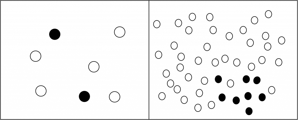
The Rare Event Problem and Imbalanced Data Sets
The rare event problem is an issue that arises frequently in churn modelling. It refers to the absolute rarity of the event being classified for inhibiting the ability of the model to learn and predict for it. This is related to, though not the same as, the problem of unbalanced datasets, where the balance of classifications skews disproportionality towards one category over another. It is possible to both have an unbalanced dataset, while still having sufficient information for the model to learn how to identify churns once rebalancing occurs.
Responses to both problems tend to be quite similar, though the optimal solution will depend on the specifics of your data (and once again may have to be determined empirically).
- Imbalanced datasets can be countered through rebalancing methods, such as under sampling. This is to be performed on the training data (for instance, making the ratio of churns to non-churns equal to 50:50), but not on the testing data.
- The rare event problem cannot be as easily resolved, since it represents an absolute, not relative, problem with the amount of churn information available. Methods of creating simulations of the data, such as over sampling, or more advanced processes like SMOTE [1] may work well. The inclusion of additional churn positive observations is typically the best counter to this problem where possible, which can often be done by refactoring the feature windows or increasing the period you’re collecting information from.
Metric to Optimise for
As with most unbalanced datasets, accuracy is not a good metric to measure for when testing the model. This is because the model simply classifying every observation as the most prevalent category would always result in a high accuracy.
While precision, recall and the F1 score are the standard alternatives, it often serves best in churn modelling (and any ML process) to liaise with key stakeholders and determine exactly what route the company intends to take to respond to the issue. This can give vital information as to what is the most important metric to optimise for.
For instance, if your retention team wants to offer discount coupons to potential churners, that would indicate that precision (how many predicted churners are actual churners) may be the most important metric, since a low precision would lead to the offering of discounts to otherwise safe users. This might even lead to users trying to take advantage of this new system if word gets out about it!
Conversely, if your retention team wants to take a more conservative approach, such as sending targeted emails, the negative impact of mis-identifying churners may be lower than not identifying actual churners. In this case, recall (what percentage of actual churners are successfully identified) would be more useful to optimise for.
Although it may seem appealing to try optimise for every metric, generally the business benefit of getting an imperfect model out quickly will far exceed that of releasing a perfect model long after it’s required. For this reason, the need for compromise and choosing carefully how to assess whether your model is “good enough” is an important consideration.
Which Algorithms to Use
As with other ML projects, which algorithm to use is often difficult to determine in advance and must be figured out empirically.
Despite this, there are some recommendations that be made. The first is to check which models are even possible to be deployed. For example, as of this time of writing Continual Integration [2] only supports nine different models like XGBoost, Catboost and RandomForest. There wouldn’t be much point using a different model that gets exceptional results, only for it not to be available at the point of deployment.
From a more churn model specific standpoint, reviews of the literature have suggested that logistic regression, SVMs and random forests work well and often held up as benchmarks. (I have tended to find that random forests work extremely well in my own churn modelling projects.)
Conclusion
That concludes the series on churn modelling! We’ve covered quite a bit, from the basis of time series data to the complexities of window selection and some of the specificities of constructing the model.
Keep in mind that churn modelling is a very broad topic, with many constantly evolving approaches to tackle it. I would highly suggest reading whatever papers you can find that look interesting if you want to dive deeper on the topic.
This is my first series of online posts made exclusively for my website. I’ll likely focus on more project-based work going forward, but if you found any of this helpful or have any suggestions for improvements, feel free to drop me a line!