
Churn Modelling Part 2:
Window Selection
“The morning rain clouds up my window” – Dido
Following on from the overview of time series data and churn modelling from Part 1, we’ll now dive into the more technical side of things with an exploration of window selection for churn modelling.
Overview of Window Segments
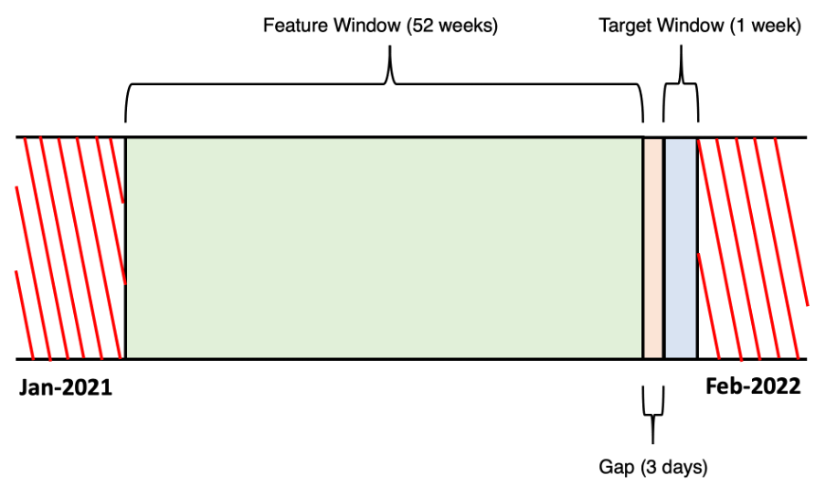
Consider a model used to predict the likelihood of an event occurring at a certain point of time in the future – for churn modelling specifically, this is whether a user will abandon the service or product.
The period in which we want to determine whether a user will churn or not is the ‘target window’. A target window might be a single recurring point of time in the future, or a critical period that the business knows in advance is approaching for each user. For example, the week prior to the auto-renewal point for a subscription is likely a critical period for voluntary churn.
The next window for consideration is a ‘gap’, or the period between when a prediction is being made and the target window period itself. The length, or even existence, of a gap will depend on business need. If the gap is too small (say you are predicting that a user will churn that very day), your retention team might not have enough time to respond effectively to the potential churner. Conversely, if you have too large a gap, you may miss out on including some of the vital data that is generated in the lead up to a user’s churn moment in your model [1].
The final window of concern is the ‘feature window’. This is the period in advance of when the prediction is being made, and from where features are extracted for inclusion in your ML model. When you tie these three windows together, you will get something like the following:

Viewing the above, the first question that may come to mind is, “what is the optimal length of each of the different windows”? And as with many great questions in ML, the answer is a resounding: “it depends”! The lengths may become obvious to you as a function of business need. For example:
- If the retention team needs at least three days to generate a targeted email offering a discount to the at-risk user, then you may require a gap period of at least three days.
- If prior analysis shows that most churns happen within a critical two-week period, then having the target window set to two weeks would ensure that this period is covered.
- If your company doesn’t store user data that is over twelve months old, than your feature window will be a maximum of twelve months (minus the gap and target window for your training data).
Realistically however, the lengths of the different window will often have to be treated much like a hyperparameter: in need of tuning to find the optimal values.
Approaches to Data Organisation for Churn Modelling
Ok, so we have a good grasp of the different windows needed for churn modelling. The next question is how the data should be constructed for the model to learn effectively on.
There are in fact many ways for you to approach this, and the best option will depend on a variety of factors, including the data you have available and the wider business needs.
Here, I’ll talk about three major approaches, taken both from my own experience and from reviews of the literature [2].
1) Single Period Aggregated Model (SPAM)
This model is probably the most common approach taken for churn modelling. This can be attributed to how simple and intuitive it is.
A single period is chosen from which the feature window, gap, and target window will be constructed. All data either side of this period is discarded.
- The target (whether the user churned or not) is extracted for every user from the target window.
- A gap is chosen for the period preceding the target window, from which all data (both response and features) is removed. A gap of zero is sometimes employed for convenience’s sake.
- The features are extracted from the remaining time that precedes the gap and is aggregated to make single-point statistics.
For example, imagine you have three years of user data from March-2019 to March-2022, including everyone’s date of churn (if they did so). You are asked to construct a model that can predict whether a user will churn or not. At least three days turn around is needed for the retention team to action a response. After considering various parameters, you decide on a set-up as follows:
In the above scenario, a period (close to the current date for freshness purposes) has been chosen. The target variables are extracted from the target window period for all users who have not churned from the start of the gap till the start of the target window. You must exclude any users who churn prior to the gap period because they do not need to be predicted for.
Within the data itself, every observation represents a user who has not churned by the start of the gap period. Information about the user is collected from the feature window and is aggregated into a point statistic. For example, the total number of times the user visited the product in the prior fifty-two weeks may be a feature, or the average duration per usage in the prior two months.
Pros and Cons
Both the advantages and disadvantages of SPAM lie in the way that it wrangles time series data into a non-time series feature space.
By restricting the period being observed, SPAM is very simple to construct out of the available data and is easy to interpret and model for. Aggregating the features into point statistics avoids the problem of constructing complex sliding feature windows which can lead to a large ratio of features to available observations. (I discuss this more in the following section.) For the above reasons, this approach is an excellent choice if you’re constrained by time and resources, or during initial explorations on how to model your data.
However, because churn modelling often suffers from the so called “rare event problem”, the number of users who churn within the chosen target window period might be too small for the model to learn effectively off. Similarly, the period chosen to model (like the last twelve months) might not be indicative of larger trends in data, such as seasonality or an unusually good or bad year. Finally, while aggregating the data does reduce the number of features and simplifies the model, it can also hide key patterns in the data, like a major drop-off in user actively in the month prior to churn.
Notes on Maintaining Model after Deployment
Because the model’s results would quickly become outdated if you never updated the training data, rolling the SPAM period forward with a frequency equal to the regularity that the model runs is necessary. For instance, a period of training data that covers Jan – June would need to become Feb – July if the model were run in the subsequent month.
2) Sliding Windows Iterative Model
This model is similar to SPAM but seeks to mitigate some of the issues inherent in the previous model by constructing periods in a constantly iterating, sliding window fashion.
Instead of having a single frame of data where every observation represents a distinct, non-churned individual, you instead construct a data-frame that is effectively a series of repeated overlapping SPAMs. This is visualised below:
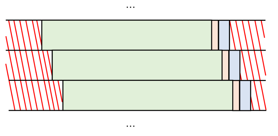
The same set up and parameters in SPAM apply as before. Because each period retains any users who are still active subscribers, a notable result of this approach is that users who do not churn in one period will reappear as observations in the subsequent one.
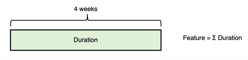
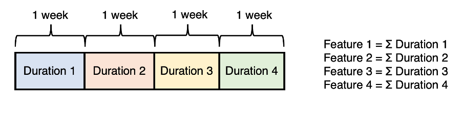
Unlike SPAM, literature on this type of model typically tends to avoid the total aggregation of features, opting for either chopping up the timeframe into smaller windows that are then aggregated, or cumulative windows stretching back over the feature window period. These three approaches are demonstrated below for the metric of duration (i.e., time spent using the product) for a feature window with a length of four weeks:
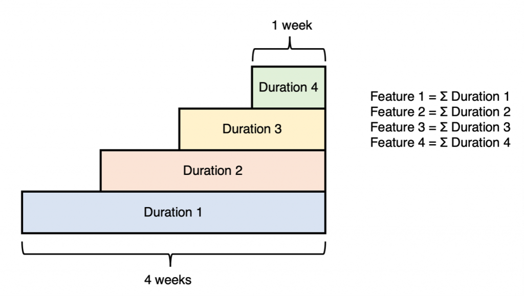
The previous two approaches to feature construction result in a much larger and more complex set of features than simple aggregation. This is usually beneficial for the model’s learning; furthermore, because SWIM supports a much larger number of observations, the n-to-p (observations to features) ratio is usually more manageable.
Pros and Cons
The biggest advantage of SWIM is that it circumvents the rare event problem by having the capacity to capture every historical churn in the company’s history, assuming the periods are backdated that far. This means that, although the data will most likely be quite imbalanced (a problem discussed in more detail in Part 3 of this blog series), there should be plenty of positive cases to learn from.
Another advantage to SWIM is that it covers much more extensive periods of time, which is especially important when accounting for seasonality. For these reasons, SWIM will likely return superior results if the time and resources for constructing and implementing it are available.
The disadvantages of the model are typically based around its size. Compared to SPAM the dataset can become very large very quickly and will continuously grow over time. This can become problematic if the time and resources required to train and implement the model aren’t available. Furthermore, depending on how dynamic the core product or service is, the model may be overweighed with old data that is no longer as relevant or useful to the modern version of the product. This problem could be mitigated by cutting off the periods used at a certain point or excluding any data older than a certain number of years.
Another issue is that the data will repeat users across multiple windows. This can lead to survivor bias, with users who go longer without churning outweighing churners who leave quickly. This may result in the development of a model that has a strong signal for identifying non-churners but a weak one for churners; an issue likely to be exacerbated by an unbalanced dataset.
Notes on Maintaining Model after Deployment
The training data for this model can be expanded by adding in whatever intervening period has passed as a new slide of data. This has the advantage of making the training data constantly grow with the most up to date (and presumably, relevant) information available.
3. Strategic Moment of Churn Model (SMOCM)
This model can be seen as a special application of SWIM. Although not as widely applicable as the other two models, which can in theory be used to detect churn at any point in the user’s lifecycle, SMOCM comes with several advantages that can maximise predictive capabilities by taking advantage of the data scientist’s knowledge of the user base.
The basic idea of SMOCM is to use predictable patterns of user churn to actively select for situations where churn can be expected, and therefore focussed on.
Let’s say you work for an online magazine service with an annual subscription model that automatically renews if the user doesn’t cancel. Although churn can technically happen anywhere within a year of a user first signing up, a distribution of voluntary churn as a function of days till end of plan would likely look something like this:
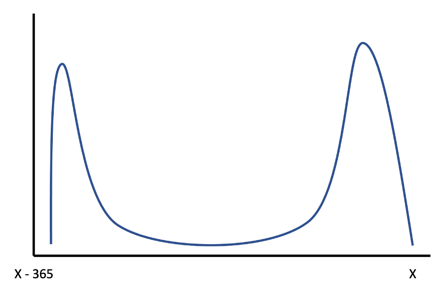
As per the above graph, many users would likely churn at the start of a plan [3], with most of the remaining doing so at the end of a plan, close to the date when they would be automatically renewed if they hadn’t cancelled.
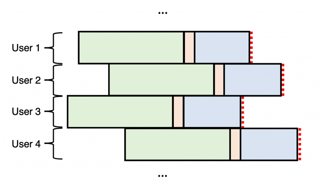
This detail significantly changes the approach we can take to construct the data for our model. Because we know in advance when a critical churn period will happen for every user (that being their final month on the plan), our periods no longer need to be selected randomly but can instead be constructed relative to every user. This can be represented diagrammatically below:
Pros and Cons
The above model seeks to employ the rigour of SWIM while discarding many of the disadvantages of continuously sliding periods.
Like SWIM, SMOCM can be backdated as far as user’s have been churning for, which can help account for seasonality [4]. Because it includes every subscription, the rare event problem is avoided since every instance of churn can be included in the model.
Although SMOCM will technically have repeated observations from users that renew their plan multiple times, these repetitions are far less than what occurs in SWIM [5]. This means that, though the amount of data used for training SMOCM is substantially greater than SPAM, it is smaller than SWIM. For these reasons, SMOCM should be the first pick when the churn period being predicted for can be narrowed down to a critical period in the user’s lifecycle.
The main disadvantage of SMOCM is that it cannot be effectively utilised as a general churn model like the other two approaches, since it requires a predicable period in a user’s lifecycle to train against.
Notes on Maintaining Model after Deployment
When deployed, the model should identify every user who falls within the target window period trained (such as the final month on their subscription plan) and classify for them only. The model should incorporate any users who pass that point (whether churned or not) as additional information for use in its training data.
Conclusion
As I hope the above has made clear, the construction of appropriate windows of data for churn modelling is an important and involved step in the ML process. A properly selected and constructed period, with good construction of the various features within it, may be the single most significant step the data scientist can take towards creating a successful model [6].
Once you have your various windows sorted out and the data organised, you now get to the fun part: constructing the model itself! Join me in Part 3 for an overview on how to deal with some of the intricacies of building a ML model in the context of churn modelling.
Here are some links to various papers that I found useful on this subject:
- How training on multiple time slices improve performance in churn prediction
- Dynamic churn prediction framework with more effective use of rare event data: The case of private banking
- Nearest-neighbor-based approach to time-series classification
[1] One additional aspect to note is: what happens if a user churns within the gap period? In this instance the model will be wrong regardless of whether it predicts the user churns or is retained, since it is only making the assessment within the target window. The best response to this issue is to try ensure the gap is as small as possible to reduce the likelihood of that happening, though the viability of this will be a function of how quickly the business can respond once the likelihood of churning has been determined. The alternative is to drop the gap to zero, with the tacit understanding that you may not have enough time to respond to a user who is predicted as likely to churn in the very near future.
[2] Note that there isn’t much of a standard for how these methods are named, so you might see similar processes named differently elsewhere.
[3] This would represent users who have no intention of resubscribing, or don’t want to remember to unsubscribe close to the end of their plan, and so cancel almost immediately after signing up.
[4] Seasonality could even be hardcoded in as a feature.
[5] Number of times renewed can be included as a feature, although you need to be careful that the association isn’t so strong that the model takes this as the main indicator. Try running the model with and without this feature to see what results you get.
[6] A heuristic or survival analysis can also be used, but having never employed either of these methods in my own churn modelling I’ll leave the reader to investigate these areas for themselves.